
Latency heatmaps are a great way to visualize latencies which are hard to grasp from pure test data. Brendan Gregg (http://brendangregg.com) has written a great Perl script for generating such heatmaps as interactive SVG graphics. Also the flamegraphs are just awesome, but this is another story.
(Unfortunately SVGs are not allowed on wordpress, so I converted this to PNG for this blog.)
Just recently I used the heatmaps to visualize the accuracy of our OPC UA Server SDKs. So this time I use this opportunity to blog about it.
I used a python test tool for measuring the sampling rate using the OPC UA timestamps. This outputs a simple list as integer values [µs since UNIX epoch].
1477661743711872
1477661743761997
1477661743811750
1477661743861417
1477661743912030
...
But for generating a heatmap you need input like that:
# time              latency
1477661743761997    50125
1477661743811750    49753
1477661743861417    49667
1477661743912030    50613
Normally when measuring services like UA read and UA write I have both values, the time when measured (sending the request) and the latency (time until I get the response from the server). This time, when measuring the sampling rate for UA monitored items this is a little bit different. I only get the timestamps when the data was sampled. I don’t care when I received the data. So I compute the latency information as the difference of two sample points.
This can simply be computed using a few lines of awk script:
BEGIN { last = 0; }
{
    if (/[0-9]+/) {
        if (last == 0) {
            last = $1;
        } else {
            latency = $1 - last;
            last = $1;
            printf "%u\t%u\n", $1, latency
        }
    }
}
The result I can feed into Brandon’s trace2heatmap.pl Perl script.
The whole process of measuring and generating the SVG is put into a simple BASH script which does the following: 1.) Calling the python test UA client 2.) Calling the awk script to prepare the data for trace2heatmap.pl 3.) Calling trace2heatmap.pl to generate the SVG
This also shows the power of Linux commandline tools like BASH, awk, and Perl. I love how these tools work seamlessly together.
Excerpt of this BASH script:
...
# do measurement
echo "Starting measurement for 10s..."
if [ $PRINT_ONLY -eq 0 ]; then
    ./test.py $URL subscription >log.txt || { cat log.txt; exit 1; }
fi
echo "Done."
# compute latency based on source timestamps
echo "Computing latency data using awk..."
awk -f latency.awk log.txt >latency.txt || exit 1
# generate heatmap
echo "Generating heatmap..."
./trace2heatmap.pl --stepsec=0.1 --unitstime=us --unitslatency=us --grid --minlat=$MINLAT --maxlat=$MAXLAT --reflat=$REFLAT --title="$TITLE" latency.txt > $SVGFILE || exit 1
echo "Done. Open $SVGFILE in your browser."
I used this to measure at 50ms sampling rate, once on Window 10, and once on Linux. The results are quiet different.
Windows 10 measurement:
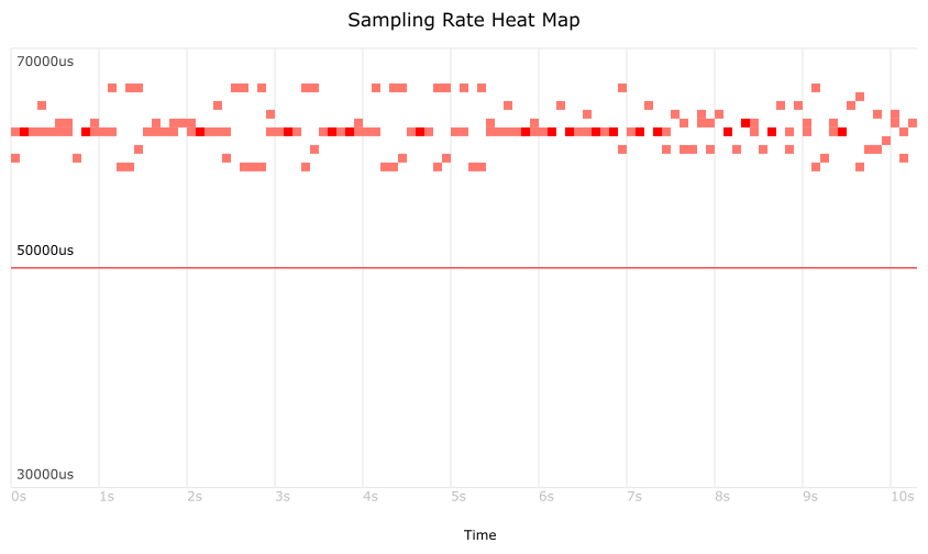
It is interesting to see that we are quiet far away from the configured 50ms sampling interval. The reason for this is that our software uses software timers for sampling that are derived from the Windows GetTickCount() API function. The resolution of this is quiet bad and is about 15-16ms. Maybe this could be improved using QueryPerformanceCounter. See also https://randomascii.wordpress.com/2013/05/09/timegettime-versus-gettickcount/
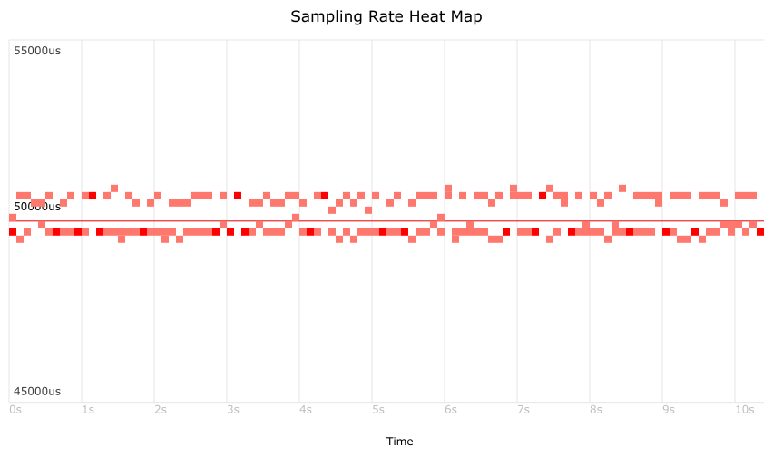
Linux measurement: (Linux ws-gergap 4.4.6-gentoo)
On Linux we use clock_gettime() to replicate the Windows GetTickCount() functionality. And this works much better. Also we don’t have such runwaway measurement results due to scheduling delays. Event though it’s a standard Linux kernel without real-time extension. Linux does a pretty good job.
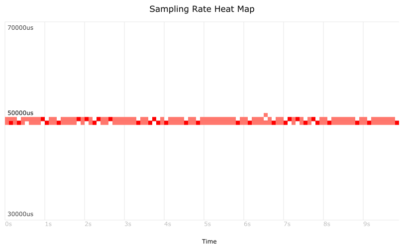
Note that both graphics above use the same scale. When zooming in more
into the Linux measurement we recognize another phenomenon:
You can see two lines in the measurement. The distance is exactly 1ms.
The reason for this is that in our platform abstraction layer we have a
tickcount() function which is modelled after the Win32 API, which means
it uses ms units. This in turn means our software cannot create more
accurate timer events, even though Linux itself would be able to handle this.
We should think about changing this to µs to get better accuracy, and maybe QueryPerformanceCounter can fix the problem also on Windows. But for the moment we are happy with the results, as they are already much better than on Windows.
2nd note: I modified the trace2heatmap.pl a little bit to show also the configured sampling rate (red line). This way it is easier to see how far away the measured timestamps are from the configured sampling rate. The Perl script is really easy to understand, so custom modifications are a no-brainer.
If somebody is interested in these scripts, just leave me a comment and I will put it on github.
Thanks to Brendan for this script and his great book and website.
Comments
comments powered by Disqus